Hierarchical Clustering - Types of Linkages

We have seen in the previous post about Hierarchical Clustering, when it is used and why. We glossed over the criteria for creating clusters through dissimilarity measure which is typically the Euclidean distance between points. There are other distances that can be used like Manhattan and Minkowski too while Euclidean is the one most often used.

There was a mention of "Single Linkages" too. The concept of linkage comes when you have more than 1 point in a cluster and the distance between this cluster and the remaining points/clusters has to be figured out to see where they belong. Linkage is a measure of the dissimilarity between clusters having multiple observations.

The types of linkages that are typically used are

1. Single Linkage

2. Complete Linkage

3. Average Linkage

4. Centroid Linkage

The type of linkage used determines the type of clusters formed and also the shape of the dendrogram.

Today we will look at what are these linkages and how do they impact the clusters formed.

Single Linkage:

Single Linkage is the way of defining the distance between two clusters as the minimum distance between the members of the two clusters. If you calculate the pair-wise distance between every point in cluster one with every point in cluster 2, the smallest distance is taken as the distance between the clusters or the dissimilarity measure.

This leads to the generation of very loose clusters which also means that the intra-cluster variance is very high. This does not give closely-knit clusters though this is used quite often.

If you take an example data set and plot the single linkage, most times you do not get a clear picture of clusters from the dendrogram.

From the plot here, you can see that the clusters don't seem so convincing though you can manage to create some clusters out of this. Only the orange cluster is quite far from the green cluster (as defined by the length of the blue line between them). Within the green cluster itself, you cannot find more clusters with a good distance between them. We will see if that is the same case using other linkages too.

As you can recollect, the greater the height (on the y-axis), the greater the distance between clusters. These heights are very high or very low between the points in the green cluster meaning that they are loosely together. Probably, they do not belong together at all.

NOTE: A part of code used to get the above dendrogram:

mergings = linkage(sample_df, method='single', metric='euclidean')
dendrogram(mergings)
plt.show()

Can we get better than this with other linkages, let us see?

Complete Linkage:

In Complete Linkage, the distance between two clusters is defined by the maximum distance between the members of the two clusters. This leads to the generation of stable and close-knit clusters.

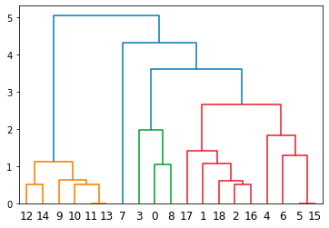
With the same data set as above, the dendrogram obtained would be like this:

Here you can see that the clusters seem more coherent and clear. The orange and green clusters are well separated. Even within the green cluster, you can create further clusters in case you want to. For example, you can cut the dendrogram at 5 to create 2 clusters within the green.

Here you can also note that the height between points in a cluster is low and between two clusters is high implying that the intra-cluster variance is low and inter-cluster variance is high, which is what we ideally want.

Note: Code used for the above dendrogram:

mergings = linkage(sample_df, method='complete', metric='euclidean')
dendrogram(mergings)
plt.show()

Average Linkage:

In Average linkage, the distance between two clusters is the average of all distances between members of two clusters. i.e.e the distance of a point from every other point in the other cluster is calculated and the average of all the distances is taken.

Using the same data set, an average linkage creates the clusters as per the dendrogram here.

Here again, you can note that the points within a suggested cluster have a very small height between them implying that they are closely knit and hence form a coherent cluster.

Note: Code used for this dendrogram:

mergings = linkage(sample_df, method='average', metric='euclidean')
dendrogram(mergings)
plt.show()

Pros and Cons:

One thing for sure is that the K-value need not be pre-defined in Hierarchical clustering. However, when you start building this tree (dendrogram), the point in one cluster cannot move. It is always in a cluster that it already belongs to and more can add to it but cannot shift clusters. Hence this is a linear method. This is a disadvantage sometimes.

Also, note that each linkage calculation is pair-wise between clusters and hence requires a huge amount of calculations to be done. The larger the data, the more the RAM, as well as the, compute power.

Between the three types of linkages mentioned above, the order of complexity of calculations is least for Single linkage and very similar for average or complete linkage.

References:

1. Order of complexity for all linkages: https://nlp.stanford.edu/IR-book/completelink.html

2. An online tool for trying different linkages with a small sample data: https://people.revoledu.com/kardi/tutorial/Clustering/Online-Hierarchical-Clustering.html

3. Single-link Hierarchical Cluster clearly explained: https://www.analyticsvidhya.com/blog/2021/06/single-link-hierarchical-clustering-clearly-explained/